Optimizers models.

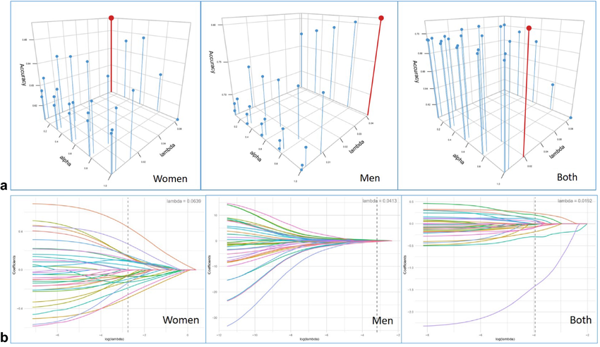
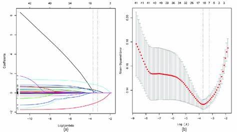
Regularization.

Regularization techniques like Lasso and Elastic Net are crucial in handling high-dimensional data, preventing overfitting, and improving model generalization.

Lasso Regression (L1 penalty) : Adds a penalty equal to the absolute value of the magnitude of coefficients. It can zero out some coefficients, effectively performing feature selection.

Elastic Net Regression (L1 and L2 penalties) Combines both L1 and L2 penalties, balancing between Lasso and Ridge regression. It’s particularly useful when dealing with correlated features.

Lasso Regression Lasso solves the optimization problem

Elastic Net Regression

Data Preparation

import numpy as np

import pandas as pd

from sklearn.model_selection import train_test_split

# Load your dataset

data = pd.read_csv('your_dataset.csv')

X = data.drop('target', axis=1)

y = data['target']

# Split the data into training and testing sets

X_train, X_test, y_train, y_test = train_test_split(X, y, test_size=0.2, random_state=42)

Advanced Feature Engineering Consider techniques like polynomial features, interaction terms, and scaling.

from sklearn.preprocessing import StandardScaler, PolynomialFeatures

# Generate polynomial and interaction features

poly = PolynomialFeatures(degree=2, include_bias=False)

X_train_poly = poly.fit_transform(X_train)

X_test_poly = poly.transform(X_test)

# Standardize the features

scaler = StandardScaler()

X_train_scaled = scaler.fit_transform(X_train_poly)

X_test_scaled = scaler.transform(X_test_poly)

Advanced Model Implementation, Lasso with Cross-Validation

Using cross-validation to find the optimal α\alphaα.

from sklearn.linear_model import LassoCV

from sklearn.metrics import mean_squared_error

# Lasso with cross-validation

lasso_cv = LassoCV(cv=10, random_state=42)

lasso_cv.fit(X_train_scaled, y_train)

# Best alpha

print(f'Optimal alpha for Lasso: {lasso_cv.alpha_}')

# Predictions and evaluation

y_pred_lasso = lasso_cv.predict(X_test_scaled)

mse_lasso = mean_squared_error(y_test, y_pred_lasso)

print(f'Lasso MSE: {mse_lasso}')

Elastic Net with Cross-Validation Using cross-validation to find the optimal

from sklearn.linear_model import ElasticNetCV

# Elastic Net with cross-validation

elastic_net_cv = ElasticNetCV(cv=10, random_state=42)

elastic_net_cv.fit(X_train_scaled, y_train)

# Best parameters

print(f'Optimal alpha for Elastic Net: {elastic_net_cv.alpha_}')

print(f'Optimal l1_ratio for Elastic Net: {elastic_net_cv.l1_ratio_}')

# Predictions and evaluation

y_pred_enet = elastic_net_cv.predict(X_test_scaled)

mse_enet = mean_squared_error(y_test, y_pred_enet)

print(f'Elastic Net MSE: {mse_enet}')

Hyperparameter Tuning using Grid Search For more granular control over hyperparameters:

from sklearn.model_selection import GridSearchCV

# Define parameter grid

param_grid = {

    'alpha': [0.01, 0.1, 1, 10, 100],

    'l1_ratio': [0.1, 0.5, 0.9]

}

# Elastic Net Grid Search

elastic_net_grid = GridSearchCV(ElasticNet(), param_grid, cv=10, scoring='neg_mean_squared_error')

elastic_net_grid.fit(X_train_scaled, y_train)

print(f'Best parameters from Grid Search: {elastic_net_grid.best_params_}')

print(f'Best score from Grid Search: {elastic_net_grid.best_score_}')

# Predictions and evaluation

best_enet = elastic_net_grid.best_estimator_

y_pred_best_enet = best_enet.predict(X_test_scaled)

mse_best_enet = mean_squared_error(y_test, y_pred_best_enet)

print(f'Best Elastic Net MSE from Grid Search: {mse_best_enet}')

Feature Selection and Model Interpretation Coefficient Analysis

After fitting the model, analyzing coefficients can help understand feature importance.

import matplotlib.pyplot as plt

# Lasso coefficients

lasso_coefs = lasso_cv.coef_

plt.plot(range(len(lasso_coefs)), lasso_coefs)

plt.title('Lasso Coefficients')

plt.show()

# Elastic Net coefficients

enet_coefs = best_enet.coef_

plt.plot(range(len(enet_coefs)), enet_coefs)

plt.title('Elastic Net Coefficients')

plt.show()

Model Deployment and Advanced Inference Saving the Model

You can use joblib to save the trained model for later use.

import joblib

# Save the best Elastic Net model

joblib.dump(best_enet, 'best_elastic_net_model.pkl')

# Load the model for inference

loaded_model = joblib.load('best_elastic_net_model.pkl')

# Make predictions with the loaded model

loaded_predictions = loaded_model.predict(X_test_scaled)

Practical Considerations Handling Multicollinearity

Elastic Net is particularly useful in the presence of multicollinearity. It can handle correlated predictors better than Lasso by combining L1 and L2 penalties.

Choosing the Right Model Lasso: Preferable when you expect a few non-zero coefficients (sparse solution). Elastic Net: Preferable when you expect many correlated features. Model Interpretation